Semi-Supervised Classification with Graph Convolutional Networks

Paper: Kipf, Thomas N.; Welling, Max. (2017). "Semi-Supervised Classification with Graph Convolutional Networks." International Conference on Learning Representations (ICLR 2017), arXiv:1609.02907. DOI: https://doi.org/10.48550/arXiv.1609.02907. Code: https://github.com/tkipf/gcn.

**GCN(Graph Convolutional Network)**은 spectral graph convolution을 1차 근사하고 self-loop가 포함된 symmetric normalization을 적용해 node feature와 graph structure를 함께 전파하는 layer-wise propagation rule을 제안한 반지도 학습 모델이다(Kipf & Welling, ICLR 2017). Citeseer 70.3%, Cora 81.5%, Pubmed 79.0%, NELL 66.0%를 기록하며 당시 주요 baseline을 상회했다.

Abstract: 본 문서는 Graph Convolutional Network(GCN)의 표준 형태를 정립한 Kipf & Welling의 ICLR 2017 논문을 해설한다. 논문의 핵심은 spectral graph convolution을 1차 근사하고 self-loop 정규화를 적용해, node feature와 graph structure를 함께 전파하는 단순한 layer-wise propagation rule을 만드는 것이다. 이 방법은 citation network와 NELL 지식 그래프 변환 데이터에서 당시 주요 semi-supervised node classification baseline보다 높은 정확도를 보고했지만, full-batch transductive 설정, undirected graph 가정, edge feature 처리의 우회적 성격을 함께 읽어야 한다.

---

Executive Summary

항목	설명
연구 질문	label이 매우 적은 graph에서 node feature와 graph structure를 함께 사용해 node class를 예측할 수 있는가?
핵심 기여	spectral graph convolution의 Chebyshev 근사를 1차로 단순화하고, self-loop가 포함된 symmetric normalization을 적용한 GCN layer를 제안한다.
방법적 결과	각 layer는 \tilde D^{-1/2}\tilde A\tilde D^{-1/2}H^{(l)}W^{(l)} 형태로 이웃 feature를 정규화 집계한 뒤 비선형 변환한다.
실험 결과	저자 보고 기준 GCN은 Citeseer 70.3%, Cora 81.5%, Pubmed 79.0%, NELL 66.0%를 기록했고, 같은 표의 Planetoid*보다 높은 정확도를 보였다.
핵심 한계	실험은 transductive full-batch 설정이다. layer 연산은 edge 수에 선형이지만, 학습 메모리와 mini-batch 확장은 논문에서 future work로 남겨졌다.

TL;DR — (1) GCN은 spectral graph convolution을 1차 근사해 \tilde D^{-1/2}\tilde A\tilde D^{-1/2}H^{(l)}W^{(l)} 형태의 단순한 layer-wise propagation으로 node feature와 graph structure를 함께 학습하는 반지도 분류 모델이다. (2) 저자 보고 기준 Citeseer 70.3%, Cora 81.5%, Pubmed 79.0%, NELL 66.0%를 달성해 Planetoid* 대비 모든 데이터셋에서 높은 정확도를 보였다. (3) 실험은 transductive full-batch 설정이며, layer 수가 늘수록 over-smoothing이 발생하고 mini-batch 확장은 future work로 남겨졌다.

목차

1. 서론
2. 예비 지식
3. 방법적 프레임워크
4. GCN layer와 2-layer 모델
5. 기존 방법과의 비교
6. 실험 결과 및 분석
7. 주의해서 읽을 점
8. 방법적 한계와 확장
9. 결론
10. References

---

1. 서론

1.1 연구 배경

GCN 논문이 다루는 문제는 graph-structured data의 semi-supervised node classification이다. 예를 들어 citation network에서는 node가 논문, edge가 인용 관계, node feature가 bag-of-words 문서 feature, label이 연구 분야가 된다. 문제는 label이 일부 node에만 있다는 점이다.

전통적인 graph-based semi-supervised learning은 대체로 "연결된 node는 같은 label을 가질 가능성이 높다"는 smoothness 가정에 기대어 label을 graph 위로 퍼뜨린다. 논문은 이 접근이 유용하지만, edge가 반드시 label similarity만 의미하지 않을 수 있다고 지적한다. 인용 관계나 지식 그래프 relation은 단순 유사도 이상을 담을 수 있다.

Kipf & Welling의 선택은 loss에 graph Laplacian regularization을 직접 추가하는 대신, 모델 자체를 adjacency matrix에 조건화하는 것이다. 즉 예측 함수 f(X, A)가 node feature X와 graph 구조 A를 함께 입력으로 받아 labeled node의 supervised loss만으로 학습된다.

1.2 핵심 질문

질문	내용
Q1	spectral graph convolution을 큰 graph에서도 쓸 수 있을 만큼 단순화할 수 있는가?
Q2	graph 구조와 node feature를 하나의 neural network layer에서 함께 전파할 수 있는가?
Q3	label이 적은 transductive node classification에서 기존 graph embedding·label propagation 계열보다 좋은 성능을 낼 수 있는가?

1.3 학술적 위치

이 논문은 GNN 연구에서 "GCN layer"라고 불리는 표준 업데이트식을 대중화한 대표 논문이다. 선행 spectral network와 ChebNet 계열이 graph Fourier/Laplacian 관점에서 convolution을 정의했다면, 이 논문은 그 복잡도를 낮추고 구현 가능한 layer rule로 정리했다. 이후의 GraphSAGE, GAT, APPNP, SGC, oversmoothing 연구 등은 대체로 이 단순한 message passing 형태를 확장하거나 비판하는 방식으로 읽을 수 있다.

다만 이 논문의 실험 설정은 오늘날 말하는 inductive representation learning 전체를 포괄하지 않는다. 논문은 full graph의 adjacency와 모든 node feature를 보는 transductive 설정에서, 일부 node label만 사용해 학습한다.

---

2. 예비 지식

2.1 Graph와 node classification

Definition 1 (Transductive node classification). 학습 시점에 전체 graph 구조와 node feature는 주어지지만, label은 일부 node에만 주어진다. 목표는 같은 graph 안의 unlabeled/test node label을 예측하는 것이다.

기호	의미
A	adjacency matrix
D	degree matrix, D_{ii}=\sum_j A_{ij}
X	node feature matrix
H^{(l)}	l번째 layer의 node representation
W^{(l)}	l번째 layer의 trainable weight
\tilde A	self-loop를 추가한 adjacency, \tilde A=A+I_N
\tilde D	\tilde A에 대한 degree matrix

2.2 Spectral graph convolution의 문제

Spectral graph convolution은 graph Laplacian의 eigenvector를 graph Fourier basis로 보고 convolution을 정의한다. 하지만 eigen-decomposition과 U matrix 곱은 큰 graph에서 비싸다. 논문은 Chebyshev polynomial approximation을 거쳐 이 계산을 localized filtering으로 바꾸고, 다시 K=1인 1차 근사로 단순화한다.

핵심 직관은 다음과 같다.

비싼 spectral convolution
  → Chebyshev polynomial로 근사
  → 1-hop 이웃만 보는 1차 filter로 단순화
  → self-loop + symmetric normalization으로 안정화
  → neural network layer로 쌓기

---

3. 방법적 프레임워크

3.1 Laplacian regularization에서 model conditioning으로

전통적 graph semi-supervised learning은 대략 다음 형태의 loss를 둔다.

이 regularization은 연결된 node의 예측이 부드럽게 변하도록 만든다. 그러나 GCN은 이 항을 loss에 직접 넣기보다, f(X,A) 자체가 adjacency를 사용하도록 만든다. labeled node에 대한 cross-entropy만 계산해도 gradient가 graph propagation 구조를 통해 unlabeled node representation에 간접적으로 영향을 미친다.

3.2 1차 근사와 renormalization trick

Chebyshev 기반 spectral convolution을 K=1로 제한하고 \lambda_{max}\approx 2로 두면, filter는 자기 자신과 정규화된 이웃 정보를 섞는 형태로 단순화된다. 논문은 parameter 수와 연산을 줄이기 위해 이를 단일 parameter 형태로 묶고, 반복 적용 시 eigenvalue 범위 때문에 생길 수 있는 numerical instability를 줄이기 위해 다음 치환을 도입한다.

여기서 \tilde A=A+I_N이다. 이 조작이 바로 논문에서 말하는 renormalization trick이다.

---

4. GCN layer와 2-layer 모델

4.1 Layer-wise propagation rule

GCN layer는 다음과 같다.

이 식은 세 부분으로 읽을 수 있다.

구성요소	역할	해석
\tilde A=A+I_N	self-loop 추가	자기 자신의 feature도 다음 representation에 남긴다.
\tilde D^{-1/2}\tilde A\tilde D^{-1/2}	symmetric normalization	degree가 큰 node의 영향이 과도해지는 것을 완화한다.
H^{(l)}W^{(l)}	feature transformation	이웃 정보를 모으기 전후로 learnable channel mixing을 수행한다.
\sigma	non-linearity	여러 layer를 쌓아 비선형 표현을 만든다.

계산 복잡도는 sparse adjacency를 쓰면 \mathcal{O}(|E|FC)로 정리된다. 여기서 C는 input channel 수, F는 output feature map 수다.

4.2 2-layer GCN

논문의 semi-supervised node classification 예시는 2-layer GCN이다.

loss는 labeled node set \mathcal{Y}_L에 대해서만 계산한다.

따라서 이 모델은 unlabeled node의 feature와 graph 위치를 representation learning에는 사용하지만, label supervision은 labeled subset에서만 받는다.

4.3 전체 흐름

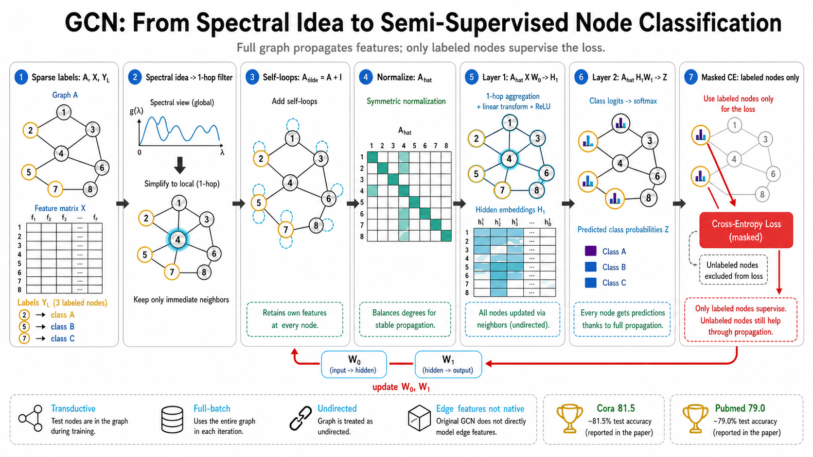
그림 1. GCN의 전체 semi-supervised training flow. 입력 그래프 A, 노드 특징 X, 일부 라벨 Y_L에서 시작해 self-loop를 추가한 \tilde{A}=A+I_N를 만들고, 대칭 정규화된 \hat{A}=\tilde{D}^{-1/2}\tilde{A}\tilde{D}^{-1/2}로 이웃 정보를 전파한다. 1층 GCN은 H^{(1)}=\mathrm{ReLU}(\hat{A}XW^{(0)})로 hidden representation을 만들고, 2층은 Z=\mathrm{softmax}(\hat{A}H^{(1)}W^{(1)})로 노드별 class probability를 예측한다. 학습 loss는 전체 노드가 아니라 라벨이 있는 노드 subset에 대해서만 cross-entropy로 계산된다. 이 그림은 원논문 figure를 재사용하지 않고, 에이전트 팀의 디자인/비판 검토를 거쳐 화이트톤 PaperBanana 스타일로 새로 생성한 자체 설명도이다. 스펙트럴 아이디어의 1-hop 단순화, self-loop와 정규화, 2-layer GCN, labeled-node-only masked loss, transductive/full-batch 한계를 한 장에 요약한다.

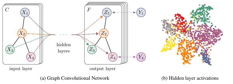
그림 2. GCN의 multi-layer 구조와 Cora hidden representation t-SNE 시각화. 왼쪽은 graph structure가 layer 전체에 공유되는 GCN 입력/출력 구조를, 오른쪽은 Cora dataset에서 label 5%를 사용해 학습한 2-layer GCN의 hidden activation을 보여준다. — Kipf & Welling (2017), Figure 1에서 연구·학습 목적상 발췌.

---

5. 기존 방법과의 비교

계열	대표 예	핵심 아이디어	GCN과의 차이
Graph Laplacian regularization	label propagation, manifold regularization	연결 node의 label/function smoothness를 loss로 강제	GCN은 loss regularizer보다 f(X,A) 구조 자체에 graph를 넣는다.
Graph embedding	DeepWalk, LINE, node2vec	random walk/skip-gram으로 node embedding을 먼저 학습	embedding 학습과 classifier 학습이 분리된 multi-step pipeline이다.
Planetoid	Yang et al. 2016	label 정보를 embedding 학습 과정에 주입	GCN은 layer propagation rule 자체로 feature와 graph를 end-to-end 결합한다.
ChebNet/spectral CNN	Defferrard et al. 2016 등	Chebyshev polynomial로 localized spectral filter 구성	GCN은 K=1 근사와 renormalization으로 더 단순한 node classification layer를 제안한다.
이전 neural graph models	recurrent GNN, diffusion CNN 등	반복적 fixed-point propagation 또는 diffusion 정의	GCN은 layer-wise feed-forward propagation과 sparse matrix multiplication으로 구현한다.

이 비교에서 중요한 점은 GCN이 완전히 새로운 "graph에서의 학습" 문제를 처음 만든 것이 아니라는 점이다. 기여는 graph-based semi-supervised learning, spectral graph theory, neural network layer 설계를 하나의 간단하고 성능 좋은 형태로 접합한 데 있다.

---

6. 실험 결과 및 분석

6.1 데이터셋과 세팅

Dataset	Type	Nodes	Edges	Classes	Features	Label rate
Citeseer	Citation network	3,327	4,732	6	3,703	0.036
Cora	Citation network	2,708	5,429	7	1,433	0.052
Pubmed	Citation network	19,717	44,338	3	500	0.003
NELL	Knowledge graph	65,755	266,144	210	5,414	0.001

Citation network에서는 class당 20개 label만 training에 사용한다. NELL은 class당 1개 labeled example이라는 더 극단적인 setting이다. 단, hyperparameter 선택에는 별도의 validation label 500개를 사용하며, test set은 1,000 labeled examples로 평가한다. 따라서 "label이 매우 적다"는 설명은 training label 기준으로 맞지만, 모델 선택에 validation label이 쓰인다는 점도 함께 적어야 한다.

6.2 주요 성능

Method	Citeseer	Cora	Pubmed	NELL
ManiReg	60.1	59.5	70.7	21.8
SemiEmb	59.6	59.0	71.1	26.7
LP	45.3	68.0	63.0	26.5
DeepWalk	43.2	67.2	65.3	58.1
ICA	69.1	75.1	73.9	23.1
Planetoid*	64.7 (26s)	75.7 (13s)	77.2 (25s)	61.9 (185s)
GCN (this paper)	70.3 (7s)	81.5 (4s)	79.0 (38s)	66.0 (48s)
GCN (rand. splits)	67.9 ± 0.5	80.1 ± 0.5	78.9 ± 0.7	58.4 ± 1.7

GCN은 Citeseer 70.3%, Cora 81.5%, Pubmed 79.0%, NELL 66.0%를 달성했다.

저자 보고 기준으로 GCN은 네 데이터셋 모두에서 Planetoid보다 높은 정확도를 보인다. 특히 Cora에서는 81.5%로 Planetoid의 75.7%보다 높고, wall-clock convergence time도 4초 대 13초로 보고된다.

그러나 이 결과는 평가된 split과 benchmark 안에서 해석해야 한다. baseline 중 ICA를 제외한 수치는 Planetoid 논문에서 가져온 것이고, random split에서 NELL의 GCN 성능은 66.0%에서 58.4 ± 1.7로 내려간다. 즉 "GCN이 항상 큰 margin으로 이긴다"가 아니라, 논문이 사용한 transductive benchmark와 split에서 강한 결과를 보고했다고 쓰는 편이 안전하다.

6.3 Propagation model ablation

Propagation model	Citeseer	Cora	Pubmed
Chebyshev filter, K=3	69.8	79.5	74.4
Chebyshev filter, K=2	69.6	81.2	73.8
1st-order model	68.3	80.0	77.5
Single parameter	69.3	79.2	77.4
Renormalization trick	70.3	81.5	79.0
1st-order term only	68.7	80.5	77.8
Multi-layer perceptron	46.5	55.1	71.4

Renormalization trick이 Citeseer 70.3%, Cora 81.5%, Pubmed 79.0%로 세 데이터셋 모두에서 가장 높은 정확도를 보였다.

Table 3은 논문의 설계 선택을 뒷받침한다. Renormalization trick은 세 citation dataset에서 가장 높은 성능을 보인다. 다만 이 결과도 해당 dataset과 architecture 안에서의 비교다. 일반적으로 모든 graph task에서 이 normalization이 최선이라고 읽으면 과장이다.

---

7. 주의해서 읽을 점

7.1 "Scalable"의 범위

논문은 layer 연산이 edge 수에 선형이라고 설명한다. 이 점은 중요한 장점이다. 하지만 학습은 full-batch gradient descent로 수행되며, 논문 스스로도 full dataset이 memory에 들어갈 때 viable하다고 말한다. Mini-batch stochastic gradient descent는 future work로 남겨졌다.

그림 3. random graph에서 edge 수가 증가할 때의 epoch당 wall-clock time. 별표는 out-of-memory error를 뜻한다. 이 그림은 GCN layer의 sparse 연산 효율성을 보여주지만, 동시에 대규모 graph에서 memory 문제가 별도 병목이 될 수 있음을 함께 읽어야 한다. — Kipf & Welling (2017), Figure 2에서 연구·학습 목적상 발췌.

따라서 실무적으로는 다음처럼 읽어야 한다.

주장	안전한 해석
GCN은 scalable하다	sparse matrix multiplication 기준 layer 연산이 edge 수에 선형이다.
GCN은 거대 graph에 바로 적용 가능하다	논문 설정만으로는 과장이다. full-batch memory, sampling, partitioning, mini-batch 설계가 추가로 필요하다.

7.2 Transductive setting

이 논문은 전체 graph 구조와 모든 node feature를 알고 있는 상태에서 일부 label만 사용하는 설정이다. 따라서 새로운 graph나 새 node가 계속 들어오는 inductive setting에 대한 직접 해답으로 읽으면 안 된다.

이 차이는 후속 연구를 이해하는 데 중요하다. GraphSAGE 같은 방법은 inductive embedding을 더 전면에 내세웠고, sampling 기반 GNN training 연구들은 full-batch GCN의 확장성 문제를 다루는 방향으로 발전했다.

7.3 Edge direction과 edge feature

논문은 기본 framework가 edge feature를 자연스럽게 지원하지 않고, undirected graph에 제한된다고 밝힌다. NELL에서는 directed labeled edge를 relation node로 바꾸는 bipartite graph 변환을 사용한다. 이는 실용적 workaround이지, edge attribute를 layer가 직접 모델링했다는 뜻은 아니다.

7.4 Homophily 가정의 완전한 제거는 아니다

GCN은 Laplacian regularization을 직접 loss에 넣지 않기 때문에, 단순 label smoothness 가정에서 한 발 벗어난다. 하지만 approximation 과정에는 여전히 locality, self-loop와 neighbor edge의 균형 같은 구조적 가정이 들어간다. heterophily graph나 edge type이 중요한 graph에서는 이 단순 평균적 aggregation이 충분하지 않을 수 있다.

---

8. 방법적 한계와 확장

8.1 논문이 밝힌 한계

한계	내용	후속 확장 방향
Full-batch memory	memory requirement가 dataset size에 선형으로 증가한다.	sampling, mini-batch, cluster/partition 기반 학습
Directed edges	기본 모델은 undirected graph를 전제로 한다.	directed GNN, relation-aware message passing
Edge features	edge attribute를 자연스럽게 처리하지 않는다.	R-GCN, edge-conditioned convolution, attention with edge features
Locality	K개 layer는 K-hop neighborhood에 의존한다.	personalized propagation, diffusion, long-range GNN
Self vs neighbor trade-off	\tilde A=A+I는 자기 자신과 이웃의 균형을 고정한다.	learnable residual/self-loop weighting

8.2 이 논문이 남긴 연구 프로그램

GCN은 이후 GNN 연구의 출발점을 다음 네 질문으로 정리하게 만들었다.

1. Aggregation: 이웃 정보를 평균할 것인가, attention으로 가중할 것인가, relation별로 다르게 처리할 것인가?
2. Scalability: full-batch를 sampling/mini-batch로 바꾸려면 어떤 approximation이 필요한가?
3. Depth: layer를 깊게 쌓으면 왜 oversmoothing이나 oversquashing이 생기는가?
4. Generalization: transductive graph 안의 node classification을 넘어 inductive node/graph/link task로 어떻게 확장할 것인가?

---

9. 결론

Kipf & Welling의 GCN 논문은 graph convolution을 대규모 node classification benchmark에서 쓰기 쉬운 neural layer로 정리했다. 핵심은 복잡한 spectral convolution을 1차 localized filter로 단순화하고, self-loop와 symmetric normalization을 통해 안정적인 propagation rule을 만든 데 있다.

이 논문을 읽을 때 가장 중요한 균형은 다음이다.

기여	읽는 법
단순하고 강한 GCN layer	이후 GNN 연구의 기본 baseline이 된 핵심 설계다.
높은 benchmark 성능	저자 보고 split과 transductive setting 안에서 강하다.
edge 수에 선형인 layer 연산	full-batch memory 문제까지 해결했다는 뜻은 아니다.
graph structure 직접 사용	edge direction/type/feature를 자연스럽게 모두 처리한다는 뜻은 아니다.

따라서 이 논문은 "모든 graph 문제의 완성형"이 아니라, graph neural network를 실용적 node classification 모델로 만든 최소하고 강력한 기준점으로 읽는 것이 가장 정확하다.

References

Kipf, T. N., & Welling, M. (2017). Semi-supervised classification with graph convolutional networks (arXiv:1609.02907). International Conference on Learning Representations. arXiv. https://arxiv.org/abs/1609.02907 (PDF 보기)

Defferrard, M., Bresson, X., & Vandergheynst, P. (2016). Convolutional neural networks on graphs with fast localized spectral filtering (arXiv:1606.09375). Advances in Neural Information Processing Systems. arXiv. https://arxiv.org/abs/1606.09375 (PDF 보기)

Yang, Z., Cohen, W. W., & Salakhutdinov, R. (2016). Revisiting semi-supervised learning with graph embeddings (arXiv:1603.08861). International Conference on Machine Learning. arXiv. https://arxiv.org/abs/1603.08861 (PDF 보기)